Experiment tracking with MLflow inside Amazon SageMaker
MLflow is a framework for end-to-end development and productionising of machine learning projects and a natural companion to Amazon SageMaker, the AWS fully managed service for data science.
MLflow solves the problem of tracking experiments evolution and deploying agnostic and fully reproducible ML scoring solutions. It lives under the Apache umbrella and is mainly supported by Databricks, the company behind Spark.
Although MLflow features integrations with some deep learning frameworks, what was definitely missing was the integration with Apache MXNet, the performance-oriented, production-ready deep learning framework.
With that in mind, I have contributed support for MXNet Gluon in MLflow. More specifically, I have added support for the Gluon interface.
I try to exemplify the features available to the MXNet and Gluon implementation in MLflow with a tutorial.
The infrastructure revolves mainly around Amazon Sagemaker and other AWS services, and while Amazon SageMaker itself features a similar solution for experiments tracking, Amazon SageMaker Experiments, I think MLflow has its advantages.
What you will learn
Here are just some of the concepts that are covered by the tutorial:
- MXNet's Gluon API for building MLP models.
- Using inference with a serialized MXNet model.
- Training in Amazon SageMaker using the Amazon SageMaker Python SDK.
- Building and using custom Docker containers for training in Amazon SageMaker.
- Logging and inspecting experiments results with MLflow.
- Using Amazon Elastic Container service.
- Creating and using a bastion server powered by OpenVPN.
- Launching and using an Amazon Aurora Serverless database.
- Configuring VPC, subnets, endpoints and security groups.
- Configuring Identity Access Management resources.
- Using AWS CLI profiles on host and in Docker guests.
The problem at hand
The supporting problem for the tutorial is identifying processes that produce Higgs bosons. The data for this is part of UCI Machine Learning Repository and detailed in Baldi, P., P. Sadowski, and D. Whiteson. “Searching for Exotic Particles in High-energy Physics with Deep Learning.” Nature Communications 5 (July 2, 2014).
I'm not going to pretend I am an expert in physics. The reason I have chosen this dataset is that it allows me to illustrate typical Machine Learning operations easily. If you are interested in finding more about the subject, you can start here.
AWS CLI
To create and manage AWS resources, you need to install and configure the AWS Command Line Interface.
- On macOS, you can use brew
brew install awscli. - On Windows, you can use Chocolatey
choco install awscli. - For Linux based systems, the official generic guidelines always works.
Once installed, the AWS CLI needs to be configured with your credentials.
Default profile
Considering that you might have several AWS CLI profiles you use, it is useful to set a default that you use for this tutorial.
In my case, I run the following command:
export AWS_PROFILE=cosmin
Account ID Environment variable
To make the rest of the snippets from the tutorial easy to copy/paste/execute, an environment variable is created. This environment variable contains the Account ID corresponding to your AWS account. This Account ID needs to be provided in several of the CLI commands you will use throughout the tutorial.
export ACC_ID=$(aws sts get-caller-identity --query Account --output text)
Running echo $ACC_ID should output your numeric Account ID without any quotes.
Prerequisites
Docker
Docker allows the creation of highly reproducible solutions utilizing fully contained containers. You can install it from here.
Optionally, you can install dry, which is a lovely utility for managing everything Docker on your local workstation. I use it often for terminating containers and check the resource usage of the individual containers.
For this tutorial, you need to have at least 8G memory allocated to Docker. Depending on your operating system, you might need to do this allocation manually, as it is the case on macOS. If you find that the Docker containers fail when processing the data later on in the tutorial, it probably means that you need to allocate even more memory. Use this to learn how to change the memory setting.
jq JSON processor
To further simplify the usage of the CLI, installing the jq JSON processor is also needed. It is available for all operating systems here. It is generally useful, and probably not a burden on your system.
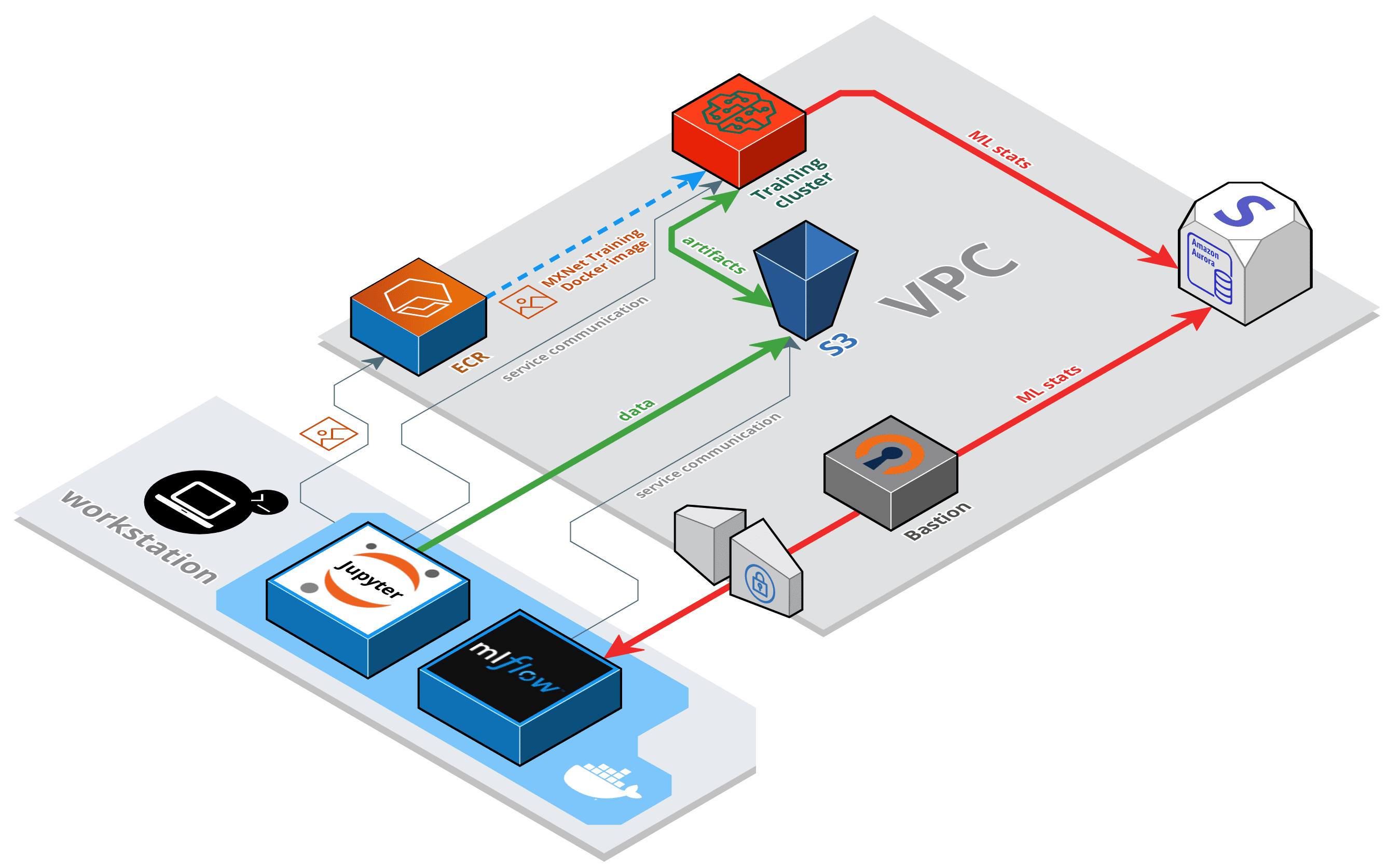
Architecture
I'm going to describe here the main parts that form the solution:
- Notebook server - this will runs on your workstation as a Docker container.
- Elastic Container Registry - this is used for storing the Docker image for training.
- Training instances - these are provisioned on-demand from the Notebook server and do the actual training of the models.
- Aurora Serverless database - the MLflow tracking data is stored in MySQL compatible, on-demand database.
- S3 bucket - Model artifacts native to SageMaker and custom to MLflow are stored securely in an S3 bucket.
- MLflow UI - The MLflow UI runs as a Docker container on your workstation.
- EC2 instance - The OpenVPN bastion facilitates access to the Aurora database.
Additionally, some IAM and VPC resources are used.

Networking Setup
Choose a VPC ID to work with
Most of the AWS resources used in this tutorial are launched inside a VPC (virtual private cloud). You should already have at least one VPC in your Amazon account, and in case you have several choose one where you would like to work in.
Listing the available VPCs can be done like this:
aws ec2 describe-vpcs | jq '.Vpcs[].VpcId' -r
You need to hold on to the VPC ID.
Choose the Subnets to work with
The VPC is actually an umbrella for subnets, which are really the important things when launching resources into VPC. You can list the subnet IDs for your VPC like this:
aws ec2 describe-subnets --filters "Name=vpc-id,Values=<YOUR VPC ID>" \
    | jq '.Subnets[] | .AvailabilityZone + "\t" + .SubnetId' -r
You need to hold on to at least two of these subnet IDs, where at least two are in different availability zones.
Create RDS subnet group
For the Aurora Database you are soon going to create, you first need to create a subnet group, which is just a wrapper around the subnets that can be used to launch the database server in. Let's just do that using the subnets you have selected in the previous step.
aws rds create-db-subnet-group \
    --subnet-ids <YOUR 1ST SUBNET> <YOUR 2ND SUBNET> \
    --db-subnet-group-name mlflow-group \
    --db-subnet-group-description "Subnets used by the MLflow db"
You need to hold on to the value mlflow-group or whatever you have chosen for the group name. This value is used when creating the Aurora database.
VPC default security group
Some of the resources you are going to launch need to be set-up with the default security group, where the term default, refers to the original default security group that comes with the creation of a VPC. Of course, the default security group can be modified, and there's nothing wrong with that, but for the sake of simplicity and to reduce the chance of unforeseen bugs, you should use a security group with the following rules:
| Direction | Source | Protocol | Port range |
|---|---|---|---|
| Inbound | The security group ID (sg-xxxxxxxx) | All | All |
| Outbound | 0.0.0.0/0 | All | All |
| Outbound | ::/0 | All | All |
To find out the default Security group ID use this:
aws ec2 describe-security-groups \
    --filters \
        Name=group-name,Values=default \
        Name=vpc-id,Values=<YOUR VPC ID> | jq '.SecurityGroups[0].GroupId' -r
If you want to confirm that the security group has not been tampered with, use this command:
aws ec2 describe-security-groups \
    --filters \
        Name=group-name,Values=default \
        Name=vpc-id,Values=<YOUR VPC ID> | jq '.SecurityGroups[0].IpPermissions'
and
aws ec2 describe-security-groups \
    --filters \
        Name=group-name,Values=default \
        Name=vpc-id,Values=<YOUR VPC ID> | jq '.SecurityGroups[0].IpPermissionsEgress'
If the default security group has been tampered with, here's how to create a new one that does what you need:
aws ec2 create-security-group \
    --group-name mlflow-default \
    --vpc-id <YOUR VPC ID> \
    --description "For MLflow tutorial"
Again, hold on to the resulting Security Group ID, this is the one you'll be using in place of the canonical default. You still need to add the rules, however.
aws ec2 authorize-security-group-ingress \
    --group-id <THE SECURITY GROUP ID YOU'VE JUST CREATED> \
    --source-group <THE SECURITY GROUP ID YOU'VE JUST CREATED> \
    --protocol all
Aurora Serverless Database
Create the database
MLflow needs to have a persistence store where results of experiments are to be kept. Choosing the persistence store needs to take into consideration that it will be used very infrequently, when training and when inspecting results. With that in mind, we look at Aurora Serverless.
The Aurora Serverless database is a MySQL compatible database that is an excellent solution for ad-hoc workloads. When the database is not in use, the resources that back it up are turned off, resulting in considerable cost savings.
This is a perfect scenario for our tutorial. It costs next to nothing to have it just lying around. It only starts costing money when you use it.
The major drawback of the serverless database is that it might not spawn up instantaneously. Especially if I choose the absolute cheapest option, I have noticed that at times I need to reissue some queries, so take note of this. Other than that, we have fewer configuration and management capabilities than with the full-flavored RDS databases. This might or might not be fine, depending on the use case.
Another vital thing to keep in mind when choosing Aurora Serverless is that direct connection to it is not possible from outside the VPC. What that means is that your workstation at home cannot connect to the database without additional effort. Aurora Serverless exposes some proprietary capabilities for remote querying, but using JDBC is not possible.
For this to work, the client connecting to the database must be in the same VPC as the database. You will see how this can be achieved in the OpenVPN Bastion section.
Here is how to spawn the database from the CLI. Quickly going through some of the arguments:
database-nameis the name of the database to be created on the server.db-cluster-identifieris the unique identifier of the server in RDS.scaling-configurationis set to the cheapest and most cost-saving conscious setting.master-username&master-user-passwordshould be set to your liking.db-subnet-group-nameis the name of the subnet group you have created in the Create RDS subnet group section.vpc-security-group-idsis the id of the default security group as described in the VPC default security group section.
aws rds create-db-cluster \
    --database-name mlflow \
    --db-cluster-identifier mlflow \
    --engine aurora \
    --engine-version 5.6.10a \
    --engine-mode serverless \
    --scaling-configuration MinCapacity=1,MaxCapacity=1,SecondsUntilAutoPause=300,AutoPause=true \
    --master-username <YOUR DB USERNAME> \
    --master-user-password <YOUR DB PASSWORD> \
    --db-subnet-group-name mlflow-group \
    --vpc-security-group-ids <YOUR DEFAULT SECURITY GROUP>
Database credentials
After finishing up creating the database, you should avoid passing the credentials to it all over the place as arguments, environment variables or the like. To do this, you can use the Secrets Manager, which is essentially a parameter store.
You create a secret with the name acme/mlflow. The breadcrumb naming is important because it allows us to control who has access to it via granular settings in Identity Access Management. This is generally useful when you don't want all the secrets in Secret Manager to be accessible to all users in your account, or all applications.
We also sneak in there the database endpoint. It just makes our life easier down the line while still keeping things consistent. To get the endpoint URL use aws rds describe-db-cluster-endpoints --db-cluster-identifier mlflow | jq '.DBClusterEndpoints[0].Endpoint' -r.
aws secretsmanager create-secret \
    --name acme/mlflow \
    --secret-string '{"username":"<YOUR DB USERNAME>", "password":"<YOUR DB PASSWORD>", "host":"<YOUR DB ENDPOINT>"}'
The secret can be configured for rotation at regular intervals with the help of a Lambda function. If you choose to do the above using the AWS Console, you have some niceties available. You can point and click your way into attaching the secret to the database directly and even configure rotation automatically via a pre-written Lambda function.
VPC Endpoints
To be able to use S3 and Secrets manager from inside the VPC, you need to create a couple of endpoints for the VPC.
The tutorial assumes that you are using us-east-1a. Please adjust if necessary.
S3
For the S3 endpoint you need the ID of the route table of your VPC.
aws ec2 describe-route-tables \
    --filters Name=vpc-id,Values=<YOUR VPC ID> Name=association.main,Values=true \
    | jq '.RouteTables[0].RouteTableId' -r
Now use it to create the endpoint.
aws ec2 create-vpc-endpoint \
    --vpc-id <YOUR VPC ID> \
    --service-name com.amazonaws.us-east-1.s3 \
    --route-table-ids <MAIN ROUTE TABLE ID>
Secrets Manager
The endpoint for Secrets Manager is as follows:
aws ec2 create-vpc-endpoint  \
    --vpc-id <YOUR VPC ID> \
    --vpc-endpoint-type Interface \
    --service-name com.amazonaws.us-east-1a.secretsmanager \
    --subnet-ids <YOUR 1ST SUBNET> <YOUR 2ND SUBNET> \
    --security-group-id <YOUR DEFAULT SECURITY GROUP>
OpenVPN Bastion
Like I have mentioned above, you cannot readily connect to the new database instance from the comfort of your home or office. What you need to do is make it seem as if you are part of the VPC the database instance lives in. To do that, you use an OpenVPN Access Server to act as a bastion for our VPC resources.
Generally speaking, a VPN server paired with a corresponding client makes it so that the traffic of the client is coming from the VPN server, that is, the VPN client assumes the IP of the VPN server. The client then gains access to, for example, resources that are covered by the canonical default security group. It should go without saying that the bastion needs to be the most secure machine in the VPC.
Another thing that the VPN server can do for us is that it can help us translate the private DNS names inside Amazon VPC. This is crucial for being able to reference the Aurora instance, which doesn't have a static IP allocated to it since it can go up and down.
Only the traffic that must go to the VPC resources should go through the bastion. I can not stress that enough. Doing otherwise can make your apparent internet connection speed slow and can end up on your AWS bill. To make sure nothing terrible happens, you will use the DNS that the bastion uses.
SSH key
To set-up the OpenVPN server, you need to connect to it via SSH. To do that, you first need to have a Key Pair configured in Amazon EC2 or create a new one.
To list available keys use this command:
aws ec2 describe-key-pairs | jq '.KeyPairs[].KeyName' -r
Just hold on to the value of one of the keys, but only if you have access to its private version as well.
If you don't have a key already, here's how to create one:
aws ec2 create-key-pair --key-name mlflow-key | jq '.KeyMaterial' -r > mlflow_key.pem
Hold on to the mlflow-key name or whatever you choose. You also need to load the private key you have just created. If you don't use Windows, it's as simple as ssh-add mlflow_key.pem. If you do use Windows, PuTTY will help.
OpenVPN security group
The OpenVPN server needs to have some ports open. You ensure that using a security group.
Note that this step is optional if you launch the OpenVPN instance using the AWS Console. I do not describe this here, though.
The command to create the needed security group is as follows. The ports are described in the OpenVPN documentation which is a good read.
aws ec2 create-security-group \
    --group-name openvpn-default \
    --vpc-id <YOUR VPC ID> \
    --description "OpenVPN default"
and the following
aws ec2 authorize-security-group-ingress \
    --group-id <THE SECURITY GROUP ID YOU'VE JUST CREATED> \
    --port 1194 \
    --protocol udp \
    --cidr 0.0.0.0/0
aws ec2 authorize-security-group-ingress \
    --group-id <THE SECURITY GROUP ID YOU'VE JUST CREATED> \
    --port 22 \
    --protocol tcp \
    --cidr 0.0.0.0/0
aws ec2 authorize-security-group-ingress \
    --group-id <THE SECURITY GROUP ID YOU'VE JUST CREATED> \
    --port 945 \
    --protocol tcp \
    --cidr 0.0.0.0/0
aws ec2 authorize-security-group-ingress \
    --group-id <THE SECURITY GROUP ID YOU'VE JUST CREATED> \
    --port 943 \
    --protocol tcp \
    --cidr 0.0.0.0/0
aws ec2 authorize-security-group-ingress \
    --group-id <THE SECURITY GROUP ID YOU'VE JUST CREATED> \
    --port 443 \
    --protocol tcp \
    --cidr 0.0.0.0/0
Launching the EC2 instance
Now it's time to actually launch the OpenVPN EC2 instance, which is as simple as:
aws run-instances \
    --image-id ami-0ca1c6f31c3fb1708 \
    --instance-type t2.nano \
    --key-name <YOUR KEY NAME> \
    --security-group-ids <YOUR OPEN VPN SECURITY GROUP> <YOUR DEFAULT SECURITY GROUP>\
    --subnet-id <YOUR 1ST SUBNET ID> \
    --associate-public-ip-address \
    --capacity-reservation-specification none \
    | jq '.Instances[0].InstanceId' -r
This gives you the InstanceId. After a few minutes, use it to get the public IP of the instance.
aws --profile cosmin ec2 describe-instances --instance-ids <THE INSTANCE ID> \
    | jq '.Reservations[0].Instances[0].PublicIpAddress' -r
It is now time to SSH into it. Once in, you are immediately presented with the OpenVPN setup. Choose the defaults. After the wizard is finished, execute sudo passwd openvpn to choose a password for the default user.
Now, go to https://<IP OF VPN SERVER> and log in. The certificate will be invalid, ignore.
Download your client and install it. Start the client.
You can now connect to private resources in VPC.
S3 bucket
You are going to need an S3 bucket to store data and artifacts in. To make things easier for Amazon SageMaker, it should be prefixed with sagemaker-. You will use this bucket for all operations involving S3.
aws s3api create-bucket \
    --bucket <YOUR BUCKET NAME STARTING WITH sagemaker-> \
    --region us-east-1
IAM execution role for Amazon SageMaker
Amazon SageMaker instances need specific permissions to be able to execute your jobs. The simplest way to create a role for this purpose is to attach the provided AmazonSageMakerFullAccess, SecretsManagerReadWrite and AmazonEC2ContainerRegistryReadOnly policies.
The permissions given are wider than what is strictly required in the tutorial, but are a good starting point.
First, you need to create a JSON document, policy.json that controls who or what can assume the created role.
{
    "Version": "2012-10-17",
    "Statement": [
        {
            "Effect": "Allow",
            "Action": [
                "sts:AssumeRole"
            ],
            "Principal": {
                "Service": "sagemaker.amazonaws.com"
            }
        }
    ]
}
Create the role:
aws iam create-role \
    --role-name <SAGEMAKER ROLE NAME> \
    --assume-role-policy-document file://policy.json \
    | jq '.Role.RoleName' -r
Now attach the Amazon managed policies:
aws iam attach-role-policy \
    --policy-arn arn:aws:iam::aws:policy/AmazonSageMakerFullAccess \
    --role-name <SAGEMAKER ROLE NAME>
aws iam attach-role-policy \
    --policy-arn arn:aws:iam::aws:policy/SecretsManagerReadWrite \
    --role-name <SAGEMAKER ROLE NAME>
aws iam attach-role-policy \
    --policy-arn arn:aws:iam::aws:policy/AmazonEC2ContainerRegistryReadOnly \
    --role-name <SAGEMAKER ROLE NAME>
Remember the Role name as you will need it in the notebook.
Running the local Jupyter notebook server
The local notebook server is a Docker based Jupyter server running in a container. Alternatively, you could be using the managed Amazon SageMaker notebook instances that come already provisioned with most packages we need.
Using a local notebook allows us to avoid some costs and not worry about starting and closing Amazon SageMaker instances, but on the other hand, data transfers are going to be slower and we need to provision the container ourselves with the needed packages. It's give and take, but it is certainly nice that the Amazon SageMaker framework does not force us into anything.
The Dockerfile you are going to be building looks like this:
FROM ubuntu:18.04

ENV DEBIAN_FRONTEND=noninteractive \
    LC_ALL=C.UTF-8 \
    LANG=C.UTF-8

RUN apt-get update && apt-get install -y --no-install-recommends \
    software-properties-common=0.96.24.32.12 && \
    add-apt-repository ppa:deadsnakes/ppa -y && \
    apt-get update && apt-get install -y --no-install-recommends \
        python3.8=3.8.2-1+bionic1 \
        python3-pip=9.0.1-2.3~ubuntu1.18.04.1 \
        build-essential=12.4ubuntu1 \
        python3-dev=3.6.7-1~18.04 && \
    rm -rf /var/lib/apt/lists/*

RUN ln -sf python3.8 /usr/bin/python
RUN pip3 --no-cache-dir install pip==20.0.2 setuptools==44.0.0

WORKDIR /

RUN pip3 install --no-cache --upgrade \
        jupyter==1.0.0 \
        mlflow==1.8.0 \
        boto3==1.12.48 \
        pandas==1.0.3 \
        scikit-learn==0.22.2.post1 \
        sagemaker==1.55.4 \
        pymysql==0.9.3 \
        mxnet==1.6.0

WORKDIR /notebooks
CMD jupyter notebook \
    --ip=0.0.0.0 \
    --allow-root \
    --no-browser \
    --NotebookApp.token='' \
    --NotebookApp.password=''
There are some comments which are valid for all Docker files used in this tutorial.
- I pin all the versions of ALL the packages I am using (both pip and aptitude), that's because I want to ensure maximum reproducibility. It's also very explicit. If there are some version issues, you'll know where to look.
- Be warned that some of the versions I have used for the Ubuntu packages (like
3.8.2-1+bionic1), might not be available at the time you might decide to reuse my code. That is because many repositories remove the old versions as they add new ones. Should that be the case, you'll need to update the versions accordingly.
Build it like docker build . -f notebook.Dockerfile -t mxnet-notebook:0.0.1.
Run it like this:
docker run \
    -p 8888:8888 \
    -v ~/.aws:/root/.aws \
    -v $(pwd)/src:/notebooks \
    -v $(pwd)/data:/notebooks/data \
    --env AWS_PROFILE=$AWS_PROFILE \
    --env ACC_ID=$ACC_ID \
    mxnet-notebook:0.0.1
You need to mount the directory containing your AWS credentials because the notebooks use it as part of the default credentials chain to authenticate against the AWS API. That is also the reason you need to provide the profile name, so that the credentials chain can figure out which profile to use.
The account ID is used as part of the following notebook.
No open a browser tab and go to localhost:8888 and create a new notebook arbiter.ipnb.
Preparing the data
The first step is, of course, to download the original raw data. It takes a few minutes to download this.
import urllib.request

src_url = "https://archive.ics.uci.edu/ml/machine-learning-databases/00280/HIGGS.csv.gz"
dest_file = "./higgs.csv.gz"
urllib.request.urlretrieve(src_url, dest_file)
Having downloaded the data, you can now load it as pandas data frame. You don't need to decompress it, pandas is able to do that under the scenes.
The usecols parameter allows us to limit the number of read columns to only the first 22. The ending 7 columns are high-level features. The whole idea with the Higgs bosons processes detection is to avoid the cumbersome job of creating these high-level features and work directly with the low-level ones, so we'll try to do just that.
The float_precision="round_trip" parameter is for making sure the there is no precision loss when writing back processed data to .csv files ref.
import pandas as pd

df = pd.read_csv(
    dest_file,
    header=None,
    usecols=list(range(0, 22)),
    float_precision="round_trip",
    names=["target"] + [f"kinematic_{i}" for i in range(1, 22)] +
          [f"high_level_feature_{i}" for i in range(1, 8)])
You will split the dataset into 3 parts: train, validation and test. The validation will be used to improve training on the training dataset and the test will give us a real-life measurement of our classifier. Do not use the test dataset for improving the training workflow, you must always choose the model with the highest value for our metric of choice, not the model with the highest resulting value against the test dataset.
You use sklearn for this. The stratify=df["target"] parameter is for making sure that the splits have the same distribution of the target variable. The test_size=.1 means that the size of the test dataset is 10% that of the whole dataset.
from sklearn.model_selection import train_test_split

train_val_df, test_df = train_test_split(df, test_size=.1,
                                         stratify=df["target"])
The train_validation_df is further separated into the final train and validation datasets.
train_df, val_df = train_test_split(train_val_df, test_size=.15,
                                    stratify=train_val_df["target"])
Now you need to persist the data frames back to disk from where you will upload them to Amazon S3. The test dataset is kept in memory for later use.
train_df.to_csv("./data/train.csv", header=False)
val_df.to_csv("./data/val.csv", header=False)
To work with Amazon Web Services, you need to initialize a session. A session allows you to initialize individual clients for different services then.
import boto3

boto3_session = boto3.session.Session(region_name="us-east-1")
You now create an Amazon SageMaker client. You use this client for uploading data to S3 and for launching powerful training clusters in the AWS cloud. Remember the S3 bucket you have created later? You need to use it here.
import sagemaker

sess = sagemaker.Session(boto3_session, default_bucket="<YOUR SAGEMAKER BUCKET>")
The Python SageMaker client is particularly powerful and versatile and some of its high-level functionality is not directly available in other languages generally supported by AWS. One of these niceties is being able to upload directly to S3 without having to instantiate an S3 client. You'll use this functionality to upload our datasets. The upload_data method returns the full S3 path to the uploaded file.
val_data_location  = sess.upload_data("./data/val.csv")
train_data_location = sess.upload_data("./data/train.csv")
Training script
In the Jupyter notebook tree, create a new Python file train.py. This script is engineered to be executed either stand-alone or in Amazon SageMaker. What you create here is the first version of the script, it will go through several iterations where it will be modified slightly.
This script is executed on Amazon SageMaker inside a container. I will explain soon how you can create a custom training container.
The code snippets have corresponding imports. If you want the whole script, you either need to take it from the complementary GitHub repository, or you can just assemble it yourself (imports at the top, of course).
Entrypoint
The channels are how Amazon SageMaker indicates the location of the various datasets (in this case, train and validation). These locations refer to the actual paths inside the container where Amazon SageMaker copies data from S3.
The MLflow secret refers to the name of the secret you have created earlier for the Aurora database. You must also provide the S3 location where model artifacts are saved to.
The last 3 parameters are actual hyperparameters for tuning the model training.
import argparse
import os

if __name__ == "__main__":
    parser = argparse.ArgumentParser()

    # Training configuration
    parser.add_argument("--train-channel", type=str,
                        default=os.getenv("SM_CHANNEL_TRAIN"))
    parser.add_argument("--validation-channel", type=str,
                        default=os.getenv("SM_CHANNEL_VALIDATION"))
    parser.add_argument("--gpus", type=int,
                        default=os.getenv("SM_NUM_GPUS"))

    # MLflow configuration
    parser.add_argument("--mlflow-secret", type=str)
    parser.add_argument("--mlflow-artifacts-location", type=str)
    parser.add_argument("--mlflow-experiment", type=str,
                        default="higgs-bosons-process-classification")

    # Actual hyperparameters
    parser.add_argument("--learning-rate", type=float, default=.01)
    parser.add_argument("--batch-size", type=int, default=128)
    parser.add_argument("--epochs", type=int, default=4)

    arguments = parser.parse_args()
    train(arguments)
Train function
The train function returns an MXNet Gluon HybridBlock.
from mxnet.gluon import HybridBlock

def train(args: argparse.Namespace) -> HybridBlock:
Getting the Aurora credentials
Here you use the Secrets Manager client created from the boto3 session to get the secret containing the database credentials for your Aurora serverless database.
You then need to set some options for the MySQL driver that is used to connect to Aurora. These are needed so that type translation happens successfully.
Finally, set the connection URI for the tracking server. This way, the MLflow library knows where to write the data.
import boto3
import mlflow
import json
import numpy as np
from pymysql import converters

session = boto3.session.Session()

client = session.client(service_name="secretsmanager", region_name="us-east-1")
mlflow_secret = client.get_secret_value(SecretId=args.mlflow_secret)
mlflowdb_conf = json.loads(mlflow_secret["SecretString"])

converters.encoders[np.float64] = converters.escape_float
converters.conversions = converters.encoders.copy()
converters.conversions.update(converters.decoders)

mlflow.set_tracking_uri(f"mysql+pymysql://{mlflowdb_conf['username']}:{mlflowdb_conf['password']@{mlflowdb_conf['host']}/mlflow")
Setting the MLflow experiment
In case the experiment already exists, you just use it, otherwise, it needs to be created and set as the active one.
if mlflow.get_experiment_by_name(args.mlflow_experiment) is None:
    mlflow.create_experiment(args.mlflow_experiment, args.mlflow_artifacts_location)
mlflow.set_experiment(args.mlflow_experiment)
Data providers
Here you load the data using pandas and then convert it to NumPy so that it can be used with the ArrayDataset class from Gluon. The Dataset objects are then used to create DataLoader objects that are really iterators over the data.
import pandas as pd
from mxnet.gluon.data import ArrayDataset, DataLoader

col_names = ["target"] + [f"kinematic_{i}" for i in range(1, 22)]

train_df = pd.read_csv(f"{args.train_channel}/train.csv.gz",
                       header=None, names=col_names)

val_df = pd.read_csv(f"{args.validation_channel}/val.csv.gz",
                     header=None, names=col_names)

train_X = train_df.drop("target", axis=1)
train_y = train_df["target"]
train_dataset = ArrayDataset(train_X.to_numpy(dtype="float32"),
                             train_y.to_numpy(dtype="float32"))
train = DataLoader(train_dataset, batch_size=args.batch_size)

val_X = val_df.drop("target", axis=1)
val_y = val_df["target"]
val_dataset = ArrayDataset(val_X.to_numpy(dtype="float32"),
                           val_y.to_numpy(dtype="float32"))
validation = DataLoader(val_dataset, batch_size=args.batch_size)
Hardware context
Amazon SageMaker will provide as argument the number of GPUs available (0 if none). The neural network and data will then be copied to the context of choice, with preference to GPU.
from mxnet import gpu, cpu

ctx = [gpu(i) for i in range(args.gpus)] if args.gpus > 0 else cpu()
MLflow magic
All tracking that follows, including artifacts and other niceties (network architecture, reproducible conda environment specifications) are due to just this little piece of code. With the help of monkey patching, you don't need to log typical values manually.
import mlflow.gluon

mlflow.gluon.autolog()
MXNet Gluon model
This is the first version of the model that you will try to improve and then select the one that performs best.
Training needs to be part of an MLflow run to be appropriately logged.
Hybridization is mandatory, otherwise MLflow cannot log the artifact, so this only works with hybridizable models.
from mxnet.gluon import Trainer
from mxnet.gluon.contrib.estimator import estimator
from mxnet.gluon.loss import SoftmaxCrossEntropyLoss
from mxnet.gluon.nn import HybridSequential, Dense, Dropout
from mxnet.initializer import Xavier
from mxnet.metric import Accuracy

with mlflow.start_run():
    net = HybridSequential()
    with net.name_scope():
        net.add(Dense(256))
        net.add(Dropout(.2))
        net.add(Dense(64))
        net.add(Dropout(.1))
        net.add(Dense(16))
        net.add(Dense(2))

    net.initialize(Xavier(magnitude=2.24), ctx=ctx)
    net.hybridize()

    trainer = Trainer(net.collect_params(), "sgd",
                      {"learning_rate": args.learning_rate})
    est = estimator.Estimator(net=net,
                              loss=SoftmaxCrossEntropyLoss(),
                              trainer=trainer,
                              train_metrics=Accuracy(),
                              context=ctx)
    est.fit(train, epochs=args.epochs, val_data=validation)

return net
Custom MXNet training image
Having finished the training script, you will now configure the training image that it will run on. Head back to your workstation's terminal.
Amazon SageMaker provides ready-made Estimators that can be used for training. These estimators are backed up by Docker images and these images are maintained by Amazon, which is great because they are of high quality. If you're just starting out, you don't want to build your own MXNet or PyTorch or TensorFlow image, you want to just start training.
However, as requirements become involved, the off-the-shelf images won't do anymore. A typical case when this happens is when you need additional libraries installed. Some of these Estimators allow for installing additional libraries by providing typical package managers' configuration files, like requirements.txt for Python packages. Still, while this might be sufficient in many cases, it won't cover more complicated cases where underlying packages need to be available. Another solution is to try to install software on-demand from your training script, such as I did in my Voice Recognition blog post, but that's also, a little bit .... "brute force".
A better idea is to provide a custom image that Amazon SageMaker can use directly, and this is the scenario I am going to explain. The advantage here is that you have full control over all the environment that is used while training.
ECR setup
Before you build the Docker image, it's good to set up the infrastructure on AWS.
You first create a Docker repository in Amazon Elastic Container Registry.
aws ecr create-repository \
    --repository-name acme/mxnet-training \
    --image-tag-mutability IMMUTABLE
This is where you will push and host your training Docker image.
Building the Docker image locally
Create a Dockerfile named mxnet-training-gpu.Dockerfile. The Dockerfile for this image is primarily based on Amazon's MXNet training image.
FROM nvidia/cuda:10.1-cudnn7-runtime-ubuntu18.04

ENV DEBIAN_FRONTEND=noninteractive \
    LC_ALL=C.UTF-8 \
    LANG=C.UTF-8

RUN apt-get update && apt-get install -y --no-install-recommends \
    software-properties-common=0.96.24.32.12 && \
    add-apt-repository ppa:deadsnakes/ppa -y && \
    apt-get update && apt-get install -y --no-install-recommends \
        build-essential=12.4ubuntu1 \
        cuda-command-line-tools-10-0 \
        cuda-cublas-10-0 \
        cuda-cufft-10-0 \
        cuda-curand-10-0 \
        cuda-cusolver-10-0 \
        cuda-cusparse-10-0 \
        ca-certificates=20180409 \
        curl=7.58.0-2ubuntu3.8 \
        wget=1.19.4-1ubuntu2.2 \
        libatlas-base-dev=3.10.3-5 \
        libcurl4-openssl-dev=7.58.0-2ubuntu3.8 \
        libgomp1=8.4.0-1ubuntu1~18.04 \
        libbz2-dev=1.0.6-8.1ubuntu0.2 \
        libopencv-dev=3.2.0+dfsg-4ubuntu0.1 \
        openssh-client=1:7.6p1-4ubuntu0.3 \
        openssh-server=1:7.6p1-4ubuntu0.3 \
        zlib1g-dev=1:1.2.11.dfsg-0ubuntu2 \
        protobuf-compiler=3.0.0-9.1ubuntu1 \
        libprotoc-dev=3.0.0-9.1ubuntu1 \
        libffi-dev=3.2.1-8 \
        cmake=3.10.2-1ubuntu2.18.04.1 \
        git=1:2.17.1-1ubuntu0.7 && \
    rm -rf /var/lib/apt/lists/*

RUN cd /usr/src && \
    curl https://www.openssl.org/source/openssl-1.0.2o.tar.gz | tar xz && \
    cd /usr/src/openssl-1.0.2o && \
    ./config --prefix=/usr/local/ssl --openssldir=/usr/local/ssl shared zlib && \
    make && make install && \
    cd /etc/ld.so.conf.d && \
    touch openssl-1.0.2o.conf && \
    echo "/usr/local/ssl/lib" > openssl-1.0.2o.conf && \
    ldconfig -v && \
    rm /usr/bin/c_rehash && rm /usr/bin/openssl

ENV PATH="${PATH}:/usr/local/ssl/bin"

RUN wget https://www.python.org/ftp/python/3.8.0/Python-3.8.0.tgz && \
        tar -xvf Python-3.8.0.tgz && cd Python-3.8.0 && \
        ./configure --enable-optimizations && \
        make && make install && \
        rm -rf ../Python-3.8.0* && \
        ln -s /usr/local/bin/pip3 /usr/bin/pip

RUN pip3 --no-cache-dir install pip==20.0.2 setuptools==42.0.2
RUN ln -s $(which python3) /usr/local/bin/python

WORKDIR /

RUN pip3 install --no-cache --upgrade --pre \
        mxnet-cu101mkl==1.6.0 \
        mlflow==1.8.0 \
        sagemaker-training==3.4.2 \
        pymysql==0.9.3 \
        pandas==1.0.3 \
        boto3==1.12.48 \
        numpy==1.18.3
I base my image on a Long Term Support Ubuntu version. The first three environment variables are used for unattended installations and encoding. The bulk of the Ubuntu packages installed are just so that you can have Python installed under a version you control. Lastly, you install the following packages:
- MXNet - we'll use it for training, it's the Cuda version for GPU.
- MLflow - we'll use it for experiment tracking.
- SageMaker Training Toolkit - utility library maintained by Amazon, which allows for easy integration with SageMaker. Without it, maintaining the image would be more cumbersome.
- PyMySQL - needed by MLflow when integrating with Amazon Aurora.
- pandas - needed for data manipulation.
- boto3 - needed for using the Secrets Manager.
- NumPy - ubiquitous library for numeric manipulations and data structures
To build the image, you just need to run a flavor of this command
docker build . -f acme/mxnet-training-gpu.Dockerfile -t acme/mxnet-training:1.6.0-gpu
mxnet-training-gpu.Dockerfile is the Dockerfile and you are in the directory where it lies. The namespace and tag acme/mxnet-training:1.6.0-gpu should be adjusted for your needs.
Once the build finishes, you need to push it to the registry in AWS.
Pushing the local image to ECR
Before being able to push the images, you need to authenticate against the registry. This is unfortunately not covered by the AWS CLI directly, as the registry works with different authentication concepts. However, the AWS CLI can be used to simplify the authentication process.
aws ecr get-login-password --region us-east-1 |\
    docker login --username AWS \
    --password-stdin $ACC_ID.dkr.ecr.us-east-1.amazonaws.com/mxnet-training
Now the local image needs to be tagged so that it matches ECR. Don't use latest for the image tag, or don't use only latest. All images should have a recognizable version. If you just use the default latest, soon you'll lose track of what image is what and won't easily be able to roll-back in case disaster hits.
docker tag acme/mxnet-training:1.6.0-gpu $ACC_ID.dkr.ecr.us-east-1.amazonaws.com/acme/mxnet-training:1.6.0-gpu
Finally, push the image remotely.
docker push $ACC_ID.dkr.ecr.us-east-1.amazonaws.com/acme/mxnet-training:1.6.0-gpu
This will take a few minutes.
Training on SageMaker
Head back to the Jupyter notebook.
Upload training artifact to S3
Training in Amazon SageMaker requires a training artifact. The training artifact must be a tar.gz file. Inside it, you put the code files needed for training.
import tarfile

with tarfile.open("model.tar.gz", mode="w:gz") as tar_gz:
    tar_gz.add("train.py")
Uploading to S3 uses the Amazon SageMaker session initialized earlier.
model_location = sess.upload_data("model.tar.gz")
Amazon SageMaker Estimator
This is the core of the SageMaker SDK, the estimator. This is where you configure how training will run. A short explanation of the parameters:
image_nameis your custom MXNet training image you have uploaded to ECR.roleis the role you have created earlier, it is used, for example, to access your secrets and work with S3.subnetsrepresents where your instances will be launched in the VPC.security_group_idsis useful because by merely having it attached, the SageMaker instances can access the Aurora Serverless database. You wouldn't usually need it otherwise.train_use_spot_instancesbecause the risks are just too small compared to the savings.hyperparametersare sent to the MXNet training container:sagemaker_submit_directoryallows you to specify the location of the training artifact.sagemaker_programallows you to specify the name of the script to execute inside the training artifact.
from sagemaker.estimator import Estimator
import os

estimator = Estimator(
    image_name=f"{os.getenv('ACC_ID')}.dkr.ecr.us-east-1.amazonaws.com/acme/mxnet-training:1.6.0-gpu",
    role="<SAGEMAKER ROLE NAME>",
    train_instance_count=1,
    train_instance_type="ml.p3.8xlarge",
    sagemaker_session=sess,
    subnets=["<YOUR 1ST SUBNET>", "<YOUR 2ND SUBNET>"],
    security_group_ids=["<YOUR DEFAULT SECURITY GROUP>"],
    train_use_spot_instances=True,
    train_max_run=12*60*60,
    train_max_wait=12*60*60,
    hyperparameters={
        "sagemaker_submit_directory": f'"{model_location}"',
        "sagemaker_program": '"train.py"',
        "mlflow-secret": '"acme/mlflow"',
        "mlflow-artifacts-location": '"s3://<YOUR SAGEMAKER BUCKET>/mlruns"',
        "epochs": "4",
        "learning-rate": "0.01"
    })
Start training
Now you do the actual launching of the Amazon SageMaker job. You provide the training and validation data as parameters.
estimator.fit(inputs={
    "train": train_data_location,
    "validation": val_data_location
})
Training will take some time.
MLflow UI
After training is done, you want to see how did your model configuration do. You will use MLflow for this.
The MLflow UI will run on your local workstation as a Docker container and will connect to both the Aurora Serverless database and S3. This is why you now need to be connected to the OpenVPN Access Server.
MLflow Docker image
This one is very basic, you only need to put a few lines in mlflow.Dockerfile:
FROM python:3.8.0

RUN pip install \
    mlflow==1.8.0 \
    pymysql==0.9.3 \
    boto3==1.12.48

CMD mlflow ui \
    --host 0.0.0.0 \
    --backend-store-uri mysql+pymysql://$USER:$PASSWORD@$HOST:3306/mlflow
and then you build it like:
build . -f mlflow.Dockerfile -t mlflow:1.8.0
Run the MLflow UI
Running the MLflow container exposes the UI on localhost:5000. Since the MLflow application need the credentials to the database, and those credentials are stored in the Secrets Manager, you can use several CLI calls to retrieve them inline. The AWS credentials are also needed because the app looks on S3 for artifacts.
docker run \
    -p 5000:5000 \
    -v ~/.aws:/root/.aws \
    --env AWS_DEFAULT_PROFILE=$AWS_PROFILE \
    --env USER=$(aws secretsmanager get-secret-value --secret-id acme/mlflow --query SecretString --output text | jq .username -r) \
    --env PASSWORD=$(aws secretsmanager get-secret-value --secret-id acme/mlflow --query SecretString --output text | jq .password -r) \
    --env HOST=$(aws secretsmanager get-secret-value --secret-id acme/mlflow --query SecretString --output text | jq .host -r) \
    --rm \
    mlflow:1.8.0
Experiments
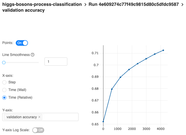
In the UI you should find a higgs-bosons-process-classification experiment and inside it your first run. It is there you can look at various metrics, such as accuracy (or your chosen metrics), loss and their values for each epoch and data set. You will use this information to assess which training configuration yields the best model in your view.
You can also find the model architecture, exported parameters and a human-readable version of the architecture. There is also a conda environment specification for the minimal requirements to run the model in an isolated environment.
If you want, as part of the training script, you can log even more metrics and parameters, it's just that you have to do that manually.
MLflow also features a bunch of integrations that help you productionize your models, be that MXNet models or something else.
ML iterations
The first iteration of the training should have an unimpressive accuracy of about .61. Let's see if it can be made higher.
When looking for the best combination of hyperparameters and network design, you go through the following steps:
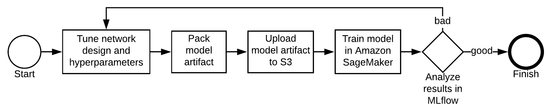
Let's do a couple more iterations and see where we get.
Second iteration
Change the training script so that your model has non-linear activations:
net = HybridSequential()
with net.name_scope():
    net.add(Dense(256, activation="relu"))
    net.add(Dropout(.2))
    net.add(Dense(64, activation="relu"))
    net.add(Dropout(.1))
    net.add(Dense(16, activation="relu"))
    net.add(Dense(2))
Also, change the hyperparameters of the SageMaker Estimator like this:
epochs8learning-rate0.01
Now, you need to re-execute the last 4 cells, starting with the one that creates the tar.gz model artifact.
Third iteration
For the last iteration, add more capacity:
net = HybridSequential()
with net.name_scope():
    net.add(Dense(512, activation="relu"))
    net.add(Dropout(.2))
    net.add(Dense(128, activation="relu"))
    net.add(Dropout(.1))
    net.add(Dense(32, activation="relu"))
    net.add(Dense(2))
Again, you need to re-execute the last 4 cells.
Choose the best model
Having 3 trials, you can now compare the performance between different configurations by analyzing the metrics inside MLflow UI. The 3rd model seems to be the best.
Another way to formally choose the best model is to search for it using the provided MLflow API. This way, you programmatically select the best member based on concrete values. Here's how to do that. Head back to the notebook.
Some of the following cell code blocks feature code from the train.py script.
To get the credentials for the tracking database, use the Secrets Manager API and then set the MLflow tracking URI.
import mlflow
import json

client = boto3_session.client(service_name="secretsmanager", region_name="us-east-1")
mlflow_secret = client.get_secret_value(SecretId="<redacted>")
mlflowdb_conf = json.loads(mlflow_secret["SecretString"])

mlflow.set_tracking_uri(f"mysql+pymysql://{mlflowdb_conf['username']}:{mlflowdb_conf['password']}@{mlflowdb_conf['host']}/mlflow")
Selecting the best model is done by sorting the runs in the Higgs Bosons experiment by validation accuracy descending.
Having the best model, you need to get the bucket and prefix key to where its artifacts are.
import re

experiment = mlflow.get_experiment_by_name("higgs-bosons-process-classification")
artifacts_location = mlflow.search_runs(experiment.experiment_id,
                                        order_by=["metrics.`validation accuracy` DESC"]).iloc[0].artifact_uri

matches = re.match(r"s3:\/\/(.+?)\/(.+)", artifacts_location)
The actual serialized model is always saved as if it is from the first epoch, hence the 0000 name suffix. You need to download the neural network architecture and its parameters.
sess.download_data(".", bucket=matches[1],
                   key_prefix=f"{matches[2]}/model/data/net-0000.params")

sess.download_data(".", bucket=matches[1],
                   key_prefix=f"{matches[2]}/model/data/net-symbol.json")
Model testing
To get the feel of how the chosen model will do in a real-life scenario, use the test data set aside to compute a final accuracy.
You initialize the model by first loading the architecture and then setting the shapes of the input. Finally, load the parameters in the network.
from mxnet import sym
from mxnet import gluon

symbol = sym.load("net-symbol.json")
net = gluon.SymbolBlock(symbol, inputs=sym.var(name="data", dtype="float32"))
net.collect_params().load("net-0000.params")
Much like in train.py, you will create the data objects allowing you to iterate the samples in the test dataset.
from mxnet.gluon.data import ArrayDataset, DataLoader

test_X = test_df.drop("target", axis=1)
test_y = test_df["target"]

test_dataset = ArrayDataset(test_X.to_numpy(dtype="float32"),
                            test_y.to_numpy(dtype="float32"))

test = DataLoader(test_dataset, batch_size=256)
Inference involves going through the test dataset in batches and executing the neural network against them.
You then use the built-in Accuracy class for storing and updating the final metric value.
from mxnet import nd
from mxnet.metric import Accuracy

metric = Accuracy()

for tensors, labels in test:
    output = net(tensors)
    predictions = nd.argmax(output, axis=1)
    metric.update(preds=predictions, labels=labels.reshape(labels.size))
The absolutely last thing you do is check the accuracy value. For me, it's around .71, which is spot on in relation to the validation test.
metric.get()
End notes
This tutorial is a mouthful. If something is not working correctly, please, get in touch with me. The link to the supporting repository is here: https://github.com/cosmincatalin/mxnet-with-mlflow-in-sagemaker.