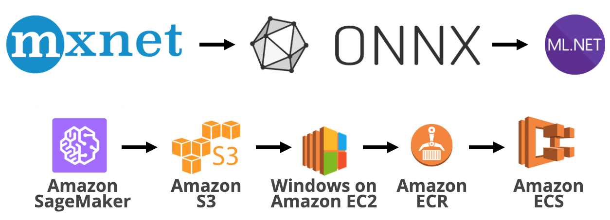
MXNet to ONNX to ML.NET with Amazon SageMaker, ECS and ECR
Data science is a mostly untapped domain in the .NET community. This is about to change, and in no small part, because Microsoft has decided to open source the ML.NET library, which can best be described as scikit-learn in .NET. The library is heavily supported with monthly releases full of features.
One of the key features of ML.NET is the ability to score using ONNX models. This is a really useful feature because it allows data scientists to work on models independently in their deep learning library of choice. The models are then converted to ONNX and used in .NET applications. One of the deep learning frameworks compatible with ONNX is Apache MXNet, which can be used to train models at scale.
However, there is a caveat, ONNX scoring only works on Windows x64 at the time of the writing.
This tutorial will show the steps necessary for training and deploying a regression application based on MXNet, ONNX and ML.NET in the Amazon Web Services ecosystem. All you need is a browser, an AWS account, and an RDP client.
Infrastructure
The infrastructure I have used for this tutorial is based on Amazon Web Services. More concretely, I have used Amazon SageMaker, ECS, ECR and EC2 services directly. A bunch of other services like VPC Networking or S3 storage are used indirectly.
Let's start with Amazon SageMaker which is used for building the initial MXNet based ONNX model. Amazon SageMaker is a service provided by Amazon which allows for developing and operationalizing machine learning projects. It is unassuming while at the same time it encourages best practices. This is a major service in the Amazon ecosystem and it receives regular updates. Some of the things that I really appreciate about it are:
- Open source machine learning algorithms ready to be used in a plug-and-play manner (Eg: XGBoost).
- Efficient use of resources.
- Hyperparameters optimization.
- Lots of hands-on tutorials on all the features of Amazon SageMaker.
From Amazon SageMaker I have used a Notebook instance where I have done the data engineering part and most of the development of the neural network training script. For the actual training job, I have used a dedicated GPU instance.
Elastic Compute Cloud was used for providing me with a Windows machine. Elastic Container Registry was used to host the Docker image which was pushed from the Windows machine.
Elastic Container Service was used to run the Windows containerized ML.NET application for inference via ONNX.
Data
The data that was used for training and testing is part of the New York Taxi Fare dataset. This will be a regression problem, as the target is a real numerical value. Since this is a proof of concept, I've only used a subset of the available dataset.
Preparing the training and test datasets
First things we need to do is have a place where we do the coding. For this purpose, we will launch a Notebook instance from the Amazon SageMaker console in AWS. An ml.m4.xlarge would be appropriate. A Notebook instance has preinstalled Jupyter with a series of kernels. We will use the Conda MXNet Python 3 kernel (conda_mxnet_p36).
After starting the notebook, we need to download the files for training and testing. These are simple .csv files.
import urllib.request

data_location = "https://raw.githubusercontent.com/cosmincatalin/mxnet-onnx-mlnet/master/data/{}"

urllib.request.urlretrieve(data_location.format("test.csv"), "test.csv");
urllib.request.urlretrieve(data_location.format("train.csv"), "train.csv");
Load the data as pandas Data Frames.
import pandas as pd

df_train = pd.read_csv("train.csv")
df_test = pd.read_csv("test.csv")
Let's take a quick look at the structure:
with pd.option_context('display.max_rows', 5, 'display.width', 1000):
    print(df_train)
which outputs
        vendor_id  rate_code  passenger_count  trip_time_in_secs  trip_distance payment_type  fare_amount
0             CMT          1                1               1271           3.80          CRD         17.5
1             CMT          1                1                474           1.50          CRD          8.0
...           ...        ...              ...                ...            ...          ...          ...
1048573       VTS          1                1               2340           4.70          CRD         24.5
1048574       VTS          1                1               1800          10.99          CSH         33.0

[1048575 rows x 7 columns]
Next step is to convert the pandas data frames to a purely numeric format. During this process, I drop the categorical features. This is so that the process can be simplified. In a real-life scenario, you would probably want to one-hot-encode or use some custom embeddings for the categorical features.
The numerical format is NDArray which is an MXNet variant of numpy. The features and target variables are separated. The features are in fact vectors.
import mxnet as mx

train_X = mx.nd.array(df_train.drop(["vendor_id", "payment_type", "fare_amount"], axis=1).values)
train_y = mx.nd.array(df_train.fare_amount.values)
test_X = mx.nd.array(df_test.drop(["vendor_id", "payment_type", "fare_amount"], axis=1).values)
test_y = mx.nd.array(df_test.fare_amount.values)
train_nd = list(zip(train_X, train_y))
test_nd = list(zip(test_X, test_y))
We define a simple function which takes the numerical data and saves it a Python pickels to a temporary location on disk.
from os import makedirs
from tempfile import gettempdir
from pickle import dump

def save_to_disk(data, type):
    makedirs("{}/pvdwgmas/data/pickles/{}".format(gettempdir(), type))
    with open("{}/pvdwgmas/data/pickles/{}/data.p".format(gettempdir(), type), "wb") as out:
        dump(data, out)
Finally, we save the data to disk, separately for training and testing.
save_to_disk(train_nd, "train")
save_to_disk(test_nd, "test")
Uploading data to S3
Once we have our train/test datasets ready, we need to upload it to S3 so that it can be made available to machines that do the actual training. For communicating with S3 and Amazon SageMaker services we will use a Amazon SageMaker client. This client has wrappers for uploading data to S3.
import sagemaker

sagemaker_session = sagemaker.Session()
Uploading is as simple as:
inputs = sagemaker_session.upload_data(
            path="{}/pvdwgmas/data/pickles".format(gettempdir()),
            bucket="redacted", key_prefix="cosmin/sagemaker/demo")
The input variable holds the S3 location where the data was uploaded.
Modeling
Modeling the Multi Layer Perceptron will happen in a separate script. The script needs to be stand alone, that is, we should be able to execute it. From the Notebook file manager, create a Python script mxnet-onnx-sagemaker-script.py.
import argparse
import os

if __name__ == "__main__":
    parser = argparse.ArgumentParser()

    parser.add_argument('--model-dir', type=str, default=os.environ["SM_MODEL_DIR"])
    parser.add_argument("--data-dir", type=str, default=os.environ["SM_CHANNEL_TRAINING"])
    parser.add_argument("--gpus", type=int, default=os.environ["SM_NUM_GPUS"])

    args, _ = parser.parse_known_args()

    model = train(args.data_dir, args.gpus)
As you can see, we use argparse to provide arguments for training. The Amazon SageMaker instance where the script will run provides a series of environment variables that can be used as defaults ref. We now need to define the train function.
from pickle import load
import mxnet as mx
from mxnet import autograd, nd, gluon
from mxnet.gluon import Trainer
from mxnet.gluon.nn import Dropout, Dense, HybridSequential
from mxnet.gluon.loss import L2Loss
from mxnet.initializer import Xavier


def train(data_dir, num_gpus):
    mx.random.seed(42)

    with open("{}/train/data.p".format(data_dir), "rb") as pickle:
        train_nd = load(pickle)
    with open("{}/test/data.p".format(data_dir), "rb") as pickle:
        test_nd = load(pickle)

    train_data = gluon.data.DataLoader(train_nd, 64, shuffle=True)
    validation_data = gluon.data.DataLoader(test_nd, 64, shuffle=True)

    net = HybridSequential()
    with net.name_scope():
        net.add(Dense(9))
        net.add(Dropout(.25))
        net.add(Dense(16))
        net.add(Dropout(.25))
        net.add(Dense(1))

    net.hybridize()

    ctx = mx.gpu() if num_gpus > 0 else mx.cpu()

    net.collect_params().initialize(Xavier(magnitude=2.24), ctx=ctx)

    loss = L2Loss()

    trainer = Trainer(net.collect_params(), optimizer="adam")

    for e in range(5):
        for i, (data, label) in enumerate(train_data):
            data = data.as_in_context(ctx)
            label = label.as_in_context(ctx)
            with autograd.record():
                output = net(data)
                loss_result = loss(output, label)
                loss_result.backward()
            trainer.step(64)

    return net
So let me go through the details of the train function:
- First we fix the random seed so that we can get reproducible results.
- Open the
picklefiles from disk. While running in Amazon SageMaker, the pickles are copied from you from where they have been uploaded in S3 to the local disk. - The numerical data from the pickles is iterated over using a dedicated iterator from MXNet Gluon,
gluon.data.DataLoader. This allows us to easily and lazily go through the data in batches. - Next comes the model. Nothing fancy here, it is a simple MLP. One thing to note here is that the model object needs to be based on
HybridSequentialwhich is a mix between imperative and symbolic, This object needs to be hybridized or changed to symbolic. - The
ctxis where training will take place. CPU, GPU or GPUs? - The network parameters are initialized using the
Xavierinitializer (a.k.a Glorot). - This is a regression problem so we can use Least Square Errors loss function.
- The
Traineris what we use to step through batches while training. Theadamoptimizer is an SGD flavored optimizer that tries to minimize the loss function. - Training takes part in the last
forloop:- We have 5 epochs, so we go through the training data 5 times.
- We take the feature and the target in batches using the lazy iterator defined above.
- In the context of
autogradwe do the forward pass - We then calculate the loss
- We do the backward pass where
autogradhelps us set the new parameter values. For the sake of simplicity, I have not included debugging information. You can find how to display the MAE in the attached gist. - We go to the next batch.
- Finally we returned the trained neural network object.
Having the model, we need to save it to disk. Amazon SageMaker will take care of uploading it to S3 afterward. So in out top-level script environment, we'll add a call to a save function
if __name__ == "__main__":
    parser = argparse.ArgumentParser()

    parser.add_argument('--model-dir', type=str, default=os.environ["SM_MODEL_DIR"])
    parser.add_argument("--data-dir", type=str, default=os.environ["SM_CHANNEL_TRAINING"])
    parser.add_argument("--gpus", type=int, default=os.environ["SM_NUM_GPUS"])

    args, _ = parser.parse_known_args()

    net = train(args.data_dir, args.gpus)
    save(net, args.model_dir)
The save function is straightforward. First, we save the MXNet model to its native format. For this, we specify the epoch for which we want to save the parameters. Second, we use the saved model to create an ONNX model that we save in the location Amazon SageMaker expects to find it. The ONNX export function needs some hints regarding the shape of the label and features that are going to be fed into the model.
from mxnet.contrib import onnx as onnx_mxnet

def save(net, model_dir):
    net.export("model", epoch=4)
    onnx_mxnet.export_model(sym="model-symbol.json",
                            params="model-0004.params",
                            input_shape=[(1, 4)],
                            input_type=np.float32,
                            onnx_file_path="{}/model.onnx".format(model_dir),
                            verbose=True)
That is it. Now it's time for the actual training. Going back to the Jupyter notebook we need to configure an Amazon SageMaker MXNet Estimator.
from sagemaker.mxnet import MXNet

estimator = MXNet("mxnet-onnx-sagemaker-script.py",
          role=sagemaker.get_execution_role(),
          train_instance_count=1,
          train_instance_type="ml.p2.xlarge",
          py_version="py3",
          framework_version="1.3.0")
The estimator needs to specify the following:
- Script file name we have defined above.
- AWS IAM role that will be used by the training machine.
- How many machines we will use for training.
- Type of machine used for training.
- The Python version.
- The MXNet version.
After this, start training:
estimator.fit(inputs)Amazon SageMaker will provision the needed resources, copy the training data to the instances and start the training process. In the end, if successful, the model artifact will be copied to S3.
For the second part of the tutorial, we will need to know where ONNX model has been copied. This information is retrieved like this:
estimator.model_dataSave the output, you will need it soon.
Provisioning the Windows machine
For this part of the tutorial, we will use Windows machine to develop a netcore application based on ML.NET. Let us begin.
Head to the EC2 console and launch a Windows with Containers instance. (I have used Microsoft Windows Server 2016 with Containers Locale English AMI provided by Amazon). You will need to connect to it via the RDP protocol, so make sure the needed port is open for connections and that you have a key you own attached to the machine. It will take a few minutes for the instance to boot up. After that, connect to it using the Remote Desktop application corresponding to your OS.
Download and install Visual Studio Code. You will need the 64-bit System Installer. The default Internet Explorer settings are a bit restrictive, but with either patience or knowledge, it is possible to use it. I had patience.
Download and install the AWS CLI 64-bit.
Download and install 7-Zip 64-bit.
Open Windows PowerShell for AWS, you can find it in the Start Menu. Change the working directory.
> cd C:\Users\Administrator\Documents\Create two folders.
> mkdir mxnet-onnx-mlnet
> mkdir mxnet-onnx-mlnet\inference
Open Visual Studio Code and open the inference folder you have just created. Here we will create 8 files.
The inference application
The project file is inference.csproj. We use netcore version 2.1. The first 3 dependencies are operational and allow us to create a web service. The Microsoft.ML.OnnxTransform is the ONNX scoring extension of ML.NET. It actually has a transient dependency on ML.NET.
<Project Sdk="Microsoft.NET.Sdk">

  <PropertyGroup>
    <OutputType>Exe</OutputType>
    <TargetFramework>netcoreapp2.1</TargetFramework>
    <StartupObject>inference.Program</StartupObject>
  </PropertyGroup>

  <ItemGroup>
    <PackageReference Include="Microsoft.AspNetCore" Version="2.1.6" />
    <PackageReference Include="Microsoft.AspNetCore.Mvc.Core" Version="2.1.3" />
    <PackageReference Include="Microsoft.AspNetCore.Mvc.Formatters.Json" Version="2.1.3" />
    <PackageReference Include="Microsoft.ML.OnnxTransform" Version="0.7.0" />
  </ItemGroup>

</Project>
The entrypoint is Program.cs. It boots up a web service that also reads configuration from the command line. This is important because that is how we will provide the path to the .onnx model file. The web service is configured via the Startup class which is next to be created.
using Microsoft.AspNetCore;
using Microsoft.AspNetCore.Hosting;
using Microsoft.Extensions.Configuration;

namespace inference
{
    internal static class Program
    {
        private static void Main(string[] args) =>
            WebHost
                .CreateDefaultBuilder()
                .ConfigureAppConfiguration((_, config) => config.AddCommandLine(args))
                .UseStartup<Startup>()
                .UseKestrel()
                .Build()
                .Run();
    }
}
The Startup.cs file makes sure we only use the absolute minimum of the MVC framework. Also, dependency injection is used to manually initialize the only controller with the prediction function.
The prediction function is what the name suggests, it is used by the controller when inference is requested. More details about it in the next paragraphs.
using inference.Controllers;
using Microsoft.AspNetCore.Builder;
using Microsoft.AspNetCore.Hosting;
using Microsoft.Extensions.Configuration;
using Microsoft.Extensions.DependencyInjection;
using Microsoft.ML;

namespace inference
{
    public class Startup
    {

        private IConfiguration Configuration { get; }

        public Startup(IConfiguration configuration)
        {
            Configuration = configuration;
        }

        public void ConfigureServices(IServiceCollection services)
        {
            services
                .AddMvcCore()
                .AddJsonFormatters()
                .AddControllersAsServices();

            var predictionFn = new Predictor(new MLContext(), Configuration.GetValue<string>("onnx")).GetPredictor();

            services.AddScoped(_ => new PredictionsController(predictionFn));
        }

        public void Configure(IApplicationBuilder app, IHostingEnvironment env) => app.UseMvcWithDefaultRoute();
    }
}
The core part of the application is the Predictor.cs file. The purpose of the Predictor class is to provide a PredictionFunction<SearchData, FlatPrediction> function that can be used to infer a numeric value (available as FlatPrediction) from a feature vector (available as SearchData).
ML.NET follows best practices in terms of machine learning pipelines and allows us to create a learning pipeline with the following instructions:
- Concatenates the
SearchDataproperties in a single vector value. - Leaves out all other values and keeps the
Features. - Uses the ONNX Scoring Estimator to infer the numerical value based on
Features. - Again, keep only the
Estimatecolumn. - Use a custom estimator to extract the numerical value from the
Estimateobject.
One thing to note is that before defining the pipeline, we had to read some data from a bogus file. This is strange, but it has to be that way for now. Because the learning pipeline needs to be fit, in theory, it also needs some data to be fit on. In practice, this pipeline is static and does not need formal fitting.
Lastly, from the Transformer that was fit, we can now extract the prediction function.
using System.IO;
using Microsoft.ML;
using Microsoft.ML.Runtime.Data;
using Microsoft.ML.Transforms;

namespace inference
{
    public class Predictor
    {
        private readonly MLContext _env;
        private readonly string _onnxFilePath;

        public Predictor(MLContext env, string onnxFilePath)
        {
            _env = env;
            _onnxFilePath = onnxFilePath;
        }

        public PredictionFunction<SearchData, FlatPrediction> GetPredictor()
        {
            var reader = TextLoader.CreateReader(_env,
                ctx => (
                    RateCode: ctx.LoadFloat(1),
                    PassengerCount: ctx.LoadFloat(2),
                    TripTime: ctx.LoadFloat(3),
                    TripDistance: ctx.LoadFloat(4)),
                separator: ',',
                hasHeader: true);
            var dummyTempFile = Path.GetTempFileName();
            var data = reader.Read(new MultiFileSource(dummyTempFile));

            var pipeline = new ColumnConcatenatingEstimator(_env, "Features", "RateCode", "PassengerCount", "TripTime", "TripDistance")
                .Append(new ColumnSelectingEstimator(_env, "Features"))
                .Append(new OnnxScoringEstimator(_env, _onnxFilePath, "Features", "Estimate"))
                .Append(new ColumnSelectingEstimator(_env, "Estimate"))
                .Append(new CustomMappingEstimator<RawPrediction, FlatPrediction>(_env, contractName: "OnnxPredictionExtractor",
                    mapAction: (input, output) =>
                    {
                        output.Estimate = input.Estimate[0];
                    }));

            var transformer = pipeline.Fit(data.AsDynamic);
            File.Delete(dummyTempFile);
            return transformer.MakePredictionFunction<SearchData, FlatPrediction>(_env);
        }
    }
}
The features that are used above are defined in the SearchData.cs file. There is a dummy property in there. It has to be there as it is used as Target variable.
using Microsoft.ML.Runtime.Api;

namespace inference
{
    public class SearchData
    {
        [ColumnName("Target")]
        public float DummyUnused{ get; set; }

        public float RateCode{ get; set; }

        public float PassengerCount{ get; set; }

        public float TripTime{ get; set; }

        public float TripDistance{ get; set; }
    }
}
The prediction output is defined in the RawPrediction.cs file:
namespace inference
{
    internal class RawPrediction
    {
        public float[] Estimate;
    }
}
The FlatPrediction is used at the end of the pipeline. The difference from the RawPrediction is that a float is used and not a vector of floats. The output of the ONNX Estimator is actually a vector of float with length 1. The definition is in the FlatPrediction.cs file:
namespace inference
{
    public class FlatPrediction
    {
        public float Estimate;
    }
}
The last project file is the PredictionsController.cs. For POST request that contains a JSON payload matching the SearchData schema, it will use the prediction function to return an estimate.
using Microsoft.AspNetCore.Mvc;
using Microsoft.ML.Runtime.Data;

namespace inference.Controllers
{
    [Route("")]
    [ApiController]
    public class PredictionsController : ControllerBase
    {
        private PredictionFunction<SearchData, FlatPrediction> _predictionFn;

        public PredictionsController(PredictionFunction<SearchData, FlatPrediction> predictionFn)
        {
            _predictionFn = predictionFn;
        }

        [HttpPost]
        public float Post([FromBody] SearchData instance) {
            return _predictionFn.Predict(instance).Estimate;
        }
    }
}
At this point the netcore application is ready.
Dockerizing the application
Create a Dockerfile in the mxnet-onnx-mlnet folder (not in the inference folder). This docker image will build the netcore application and it will pack the ONNX model file inside the image along with the application artifact and all the dependencies needed to run it. Note that this is Windows container image. It needs to run on a version of Docker that runs Windows containers. This is only possible in Windows.
FROM microsoft/dotnet:sdk AS build-env
COPY inference/*.csproj /src/
COPY inference/*.cs /src/
WORKDIR /src
RUN dotnet restore --verbosity normal
RUN dotnet publish -c Release -o /app/ -r win10-x64

FROM microsoft/dotnet:aspnetcore-runtime
COPY --from=build-env /app/ /app/
COPY models/model.onnx /models/
COPY lib/* /app/
WORKDIR /app
CMD ["dotnet", "inference.dll", "--onnx", "/models/model.onnx"]
Back in the PowerShell terminal, make sure that you are in the mxnet-onnx-mlnet folder. First, upgrade docker.
> Install-Package -Name Docker -ProviderName DockerMsftProvider -Force -VerboseRestart
> Restart-service dockerNow it is time to make use of the AWS CLI. Again, make sure that the PowerShell you are using is the AWS one. Let us proceed.
> mkdir models
> cd models
> aws s3 cp s3://redacted/sagemaker-mxnet-2018-12-04-12-19-28-732/output/model.tar.gz .
Instead of the dummy S3 path I have used above, use the output of estimator.model_data, the last cell in the Python Jupyter notebook.
The ONNX model is now on our Windows instance. Use Windows Explorer and 7-Zip to extract it to the same folder. You should end up with something like this:
> dir C:\Users\Administrator\Documents\mxnet-onnx-mlnet\models


    Directory: C:\Users\Administrator\Documents\mxnet-onnx-mlnet\models


Mode                LastWriteTime         Length Name
----                -------------         ------ ----
-a----        12/4/2018  12:30 PM           2432 model.onnx
-a----        12/4/2018  12:30 PM          10240 model.tar
-a----        12/4/2018  12:30 PM           1434 model.tar.gz
What we're interested in the model.onnx. As long as that's in the models/ folder, we're good.
We will create a repository in ECR from the command line and we will push our new image to it.
> aws ecr create-repository --repository-name acme/onnx --region us-east-1You should get an output similar to the following:
{
    "repository": {
        "repositoryArn": "arn:aws:ecr:us-east-1:redacted:repository/acme/onnx",
        "registryId": "redacted",
        "repositoryName": "acme/onnx",
        "repositoryUri": "redacted.dkr.ecr.us-east-1.amazonaws.com/acme/onnx",
        "createdAt": 1544268380.0
    }
}
Then build the image that will hold the inference application.
> docker build -t mxnet-onnx-mlnet .Now we need to retrieve the login command to use to authenticate the Docker client to the registry
> Invoke-Expression -Command (Get-ECRLoginCommand -Region us-east-1).CommandThe output of the above command must finish with Login Succeeded.
Next, we will tag the image. Replace the url I use with the output that you get for repositoryUri above.
> docker tag mxnet-onnx-mlnet:latest redacted.dkr.ecr.us-east-1.amazonaws.com/acme/onnx:latestFinally, we are going to push the image t the repository.
> docker push redacted.dkr.ecr.us-east-1.amazonaws.com/acme/onnx:latestWe are done with the Windows machine. It can be terminated.
Running the application in Elastic Container Service
To be able to run our application we will need to head to the ECS console.
Creating an ECS Task
- Go to Task Definitions and start creating a new one.
- Choose type compatibility EC2.
- For Task Definition Name put something like onnx.
- Leave everything else as it is and fill in 1024 for Task Memory and 1 vcpu for Task CPU.
- Add a container.
- For Container Name put something like onnx.
- For Image you need to fill in the
repositoryUriabove (Eg:redacted.dkr.ecr.us-east-1.amazonaws.com/acme/onnx). - Add port mapping host:
5000to container:80. - In the Storage and Logging section, choose awslogs for Log configuration. This will help in case things go wrong.
- Leave everything else as it is and save.
- Leave everything else as it is and click on Create.
Your task definition is ready. We will now create a cluster to run our Docker container.
Creating an ECS Cluster
- Go to Clusters and create a new cluster.
- Choose the EC2 Windows + Networking template.
- For Cluster name choose something like win-docker-cluster.
- Choose a t2.medium for EC2 instance type.
- In the Networking section, choose one of your VPNs. You need to have one.
- Choose a subnet that auto-assigns
IPv4. This can be enabled in the VPC console. - Choose a sensible security group, but make sure that the EC2 machine is able to talk to the ECS service. In practice, if your security group just allows all connections from inside the VPC, it should work and be moderately safe at the same time.
- Lastly, for the Container instance IAM role choose ecsInstanceRole.
- Finish by pressing on Create.
- In a few minutes (10ish), you should have a cluster ready to run Windows docker containers.
Run the Application
Once you see something in the ECS Instances tab of your cluster you can proceed to the next step, running the application.
- Go to the Tasks tab available in your clusters management console
- Click on Run new Task.
- Choose type EC2.
- Task definition should correspond to what you have defined earlier in the Task section, in my case that would be onnx:1 (where 1 stands for the version of the task, you probably want the latest one).
- Leave everything else as it is and run the task.
- The container should be ready in a couple of minutes. The Last Status must be RUNNING.
That's it, we're done. You can now use the containerized application for inference. Let's test that.
Testing the endpoint
The application is running, but to access it you need its IP. In the ECS cluster corresponding to your application go to the Tasks tab and click on your running application. In the new page that opens, expand the details of the onnx container. In the Network bindings section you will see an IP of the form xxx.xxx.xxx.xxx:5000. Copy just the value of the IP. Go to the EC2 console and open the Instances listing. Search for the copied IP and a single instance should be listed. In its details, you will see the Private IPs. That is what you want. Copy it and save it somewhere. We will use it next.
To test the application we need an EC2 instance that runs in the same VPC as the ECS cluster. Also, the EC2 must have the security groups assigned so that the ECS cluster allows connection to it. Launch such a Linux based EC2 instance and be sure you can connect to it via SSH.
After you connect to the test EC2 machine run the following cURL command:
> curl -H "Content-Type: application/json" -d "{'RateCode':1.0,'PassengerCount':1.0,'TripTime':1.0,'TripDistance':1.0}" xxx.xxx.xxx.xxx:5000Be sure to replace xxx.xxx.xxx.xxx:5000 with the value you have copied above for the private IP. Running the above cURL command must get you back something very close to 4.3895 as a result.